Within the last two years, there has been a dramatic surge of research in randomized numerical linear algebra focused on designing efficient algorithms for working with tensors rather than just matrices.

As a researcher in this area, I have felt this shift directly in the volume of relevant weekly arXiv posts related to tensors. I wanted to see whether that intuition could be quantified.

Google recently released Google Trends, which is a nifty tool for tracking how search activity for a topic changes over time. To quantify the rise in tensor-related interest, I collected monthly relative search-volume data (case-insensitive) for the query keywords Tensor network, Tensor decomposition, Tensor Train, Matrix Product State, and Random tensor over the past ten years. I then fit an RBF-kernel Gaussian process and tuned its hyperparameters with an L-BFGS optimizer to regress the data. The results speak for themselves:

This shift toward tensor-structured linear algebra computation was anticipated in a punchy 1999 research article, “The Ubiquitous Kronecker Product” [1], in which Charles Van Loan (of Matrix Computations [2] fame) argues that algorithms organized around tensor structure would pave the path forward for the next (now current) generation of scientific computing. As active research topics like quantum information and machine learning continue to bleed into the applied mathematics purview, it seems Van Loan’s prediction is finally coming true.

While it is fantastic that more and more people are becoming interested in tensors, one recurring response I hear from applied mathematicians is that tensor papers are often hard to read and sometimes outright confusing. I share this feeling, and I believe the main contributing factor is the lack of a standardized tensor syntax.

To get a sense of how widespread this issue is, I asked the following question to some of my friends in the randomized linear algebra community.

These were the responses I received:

Each of these individuals is a fantastic researcher in numerical linear algebra. Even so, there is clearly a substantial barrier to entry for working with tensors.

This blog post is the first entry of a series called Seeing Is Believing, so it’s only fair that I show you what this actually looks like:

Writing out the basis expansion of a single tensor is really not that bad. It even gives us an excuse to use $\texttt{\bigotimes}$, which is always fun. The real issues start to appear when we reason about operations between tensors, such as the (tensor) Kronecker product. Given an order-$n$ tensor $\tX\in \Rdtensor{n}$ and an order-$m$ tensor $\tY \in \Rdtensor{m}$, even writing down what this operator does requires at least $m+n+5$ unique variables.

Recall that when the tensors are just matrices $\mA \in \bbR^{m \times n}$ and $\mB \in \bbR^{p \times q}$, their Kronecker product is the block matrix

The tensor Kronecker product follows the same principle: entries of one tensor scale full copies of the other. We return to a full definition of this operation later (Jump to the definition) for now though, we can take a peek at what this looks like:

“Index blow-up” is so pervasive that many texts about tensors open with some form of cautionary remark informing the reader that there are rough waters ahead.

“In tensor calculations the maze of indices often makes one lose sight of the very great differences between various types of quantities which can be represented by tensors.”

— Harley Flanders, Differential Forms with Applications to the Physical Sciences [3], 1989, Foreword p. 5

It’s a sad state of affairs when each time a reader sits down with this type of mathematics that a preceding Goosebumps style warning is necessary.

To make matters worse, at the frontier of tensor and tensor-network research, even writing down fully rigorous proofs (for example, approximation guarantees) can become very hard to parse without a second monitor and some emotional support coffee.

Really, this blog post is an unabashed love letter to a (partial) solution to the syntactic challenges of working with tensors called Penrose Diagrams.

Like many of us, after a sufficient investment of time, Nobel Laureate Sir Roger Penrose eventually became exhausted with explicit tensor syntax. Unlike many of us, he then proceeded to create an entirely new way of thinking about tensors. His motivation (and frustration) is best captured in his prefacing comments before introducing his diagram notation for the first time in the 1971 paper Applications of Negative Dimensional Tensors [5].

“…Even in the case of ordinary finite dimensional systems we can retain the full flexibility and simplicity of the tensor index notation while eliminating the undesirable basis dependence of the usual notation.

However the above is still subject to the other criticism which is sometimes levelled at such index notations, namely the fact that with many indices, expressions may become cumbersome and all-important index connections are easily misread.

I shall therefore introduce a diagrammatic notation for tensors which in most instances allows connections between indices to be discerned at a glance. (mic drop)”

— Sir Roger Penrose, Applications of Negative Dimensional Tensors, 1971, pg 224

I tried reaching out to Sir Roger Penrose to ask him personally about his thoughts on tensor networks, but received the following response:

$\texttt{This is an automated message}$.

Roger Penrose no longer reads this mailbox.

… Roger is over 90 years old and has much reduced capacity to engage with the wide range of people that still wish to communicate with him.

If you have not heard back within 3 months you are unlikely to do so.

That was about two months ago, so it’s unlikely we’ll find out anytime soon (if ever ☹).

In the remainder of this blog post, I will make the claim that not only are Penrose diagrams the fastest way to reason about tensor contraction, but they are also the best tool for designing tensor network algorithms, since they can reveal the computational complexity of a given method by inspection.

Penrose diagrams are fairly easy to explain but a little more challenging to fully understand. We will start by investing some energy in understanding the two basic tensor operations (the Kronecker product and partial trace) so that tensor contraction can be defined as a one-liner. For additional excellent refreshers on tensor diagrams, see [7, Sec. 3.83], [8, Sec. 2] or [6],[9] which are each beautiful passes on this topic.

Just Draw Circles

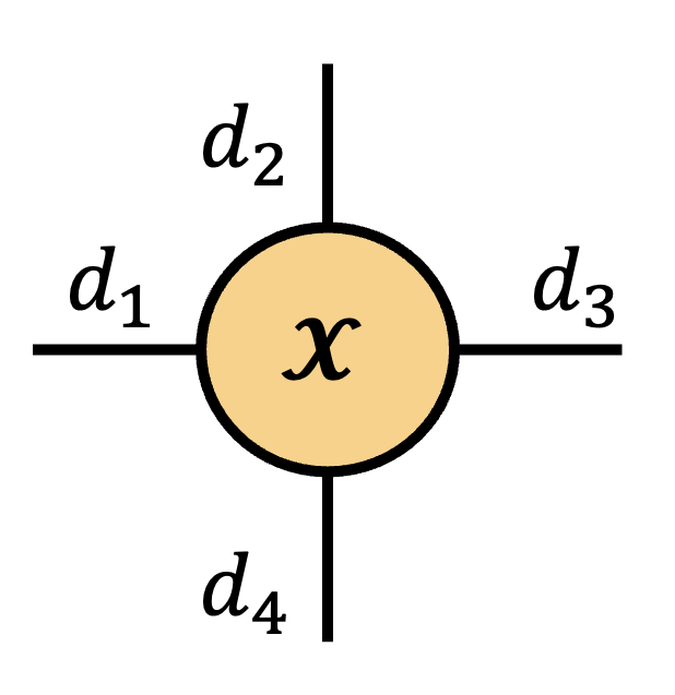
Visually, Penrose diagrams are extremely simple. All tensors are drawn as an arbitrary shape, often a circle, with an edge or leg emanating outward for each mode of the tensor. For example, this is how to draw a order 1,2, and three tensor.

The length and orientation of each leg is also arbitrary, and is generally drawn in whatever way makes it easier to understand what’s going on. Depending on the setting, the shape of a node may be changed from a circle to some other shape to reflect additional structure or set it apart from other tensors.

The Investment: Representing Tensor Contraction

So far, we have mostly just drawn circles and lines. We start to collect dividends once we use this notation to represent contractions.

The main purpose of Penrose diagrams is to reduce the time required to reason about tensor contraction.

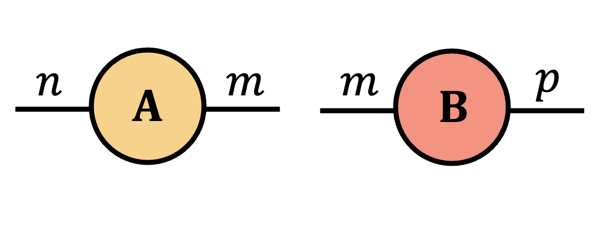
In a Penrose diagram to contract two tensors along a shared mode, you simply connect the corresponding legs with a line. For example, here are a few softballs from familiar linear algebra settings.

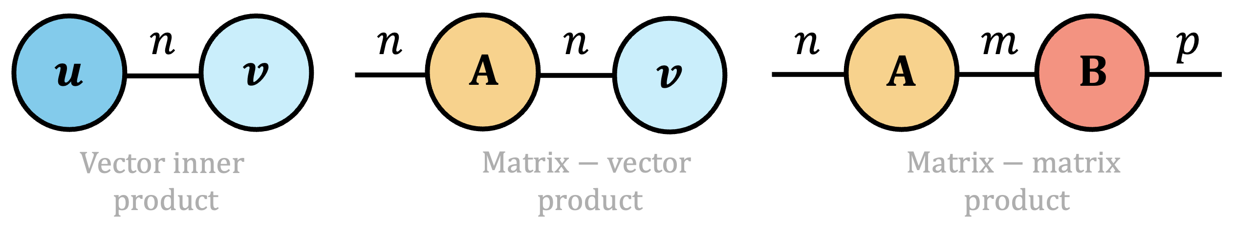
We can extend this idea to include contractions among much larger sets of tensors as well. In the following example, we consider contracting a $3\times 4$ grid of $12$ different tensors together to see how much effort we are saving.

Where we are headed: Penrose notation vs. traditional syntax

Traditional syntax

---

Let $V \simeq \bbR^{d}$ and $H \simeq \bbR^{\chi}$, with bases $\{\ve_a\}_{a=1}^{d}, \{\vf_a\}_{a=1}^{d}\subset V$ and $\{\vg_{\alpha}\}_{\alpha=1}^{\chi}, \{\vh_{\alpha}\}_{\alpha=1}^{\chi}\subset H$. Define indicies $$ \begin{aligned} t_i,u_i,s_i&\in\{1,\dots,d\},\\ \alpha_i,\beta_i,\gamma_i&\in\{1,\dots,\chi\}. \end{aligned} $$ $$ \alpha_0=\alpha_4=\beta_0=\beta_4=\gamma_0=\gamma_4=1. $$ For each site $i\in\{1,2,3,4\}$, define the following tensors: $$ A_i = \sum_{t_i=1}^{d}\sum_{u_i=1}^{d}\sum_{\alpha_{i-1}=1}^{\chi}\sum_{\alpha_i=1}^{\chi} A_i(t_i,u_i,\alpha_{i-1},\alpha_i)\, \bigl(\ve_{t_i}\otimes \vf_{u_i}\otimes \vg_{\alpha_i}\otimes \vh_{\alpha_{i-1}}\bigr). $$ $$ B_i = \sum_{u_i=1}^{d}\sum_{s_i=1}^{d}\sum_{\beta_{i-1}=1}^{\chi}\sum_{\beta_i=1}^{\chi} B_i(u_i,s_i,\beta_{i-1},\beta_i)\, \bigl(\ve_{u_i}\otimes \vf_{s_i}\otimes \vg_{\beta_i}\otimes \vh_{\beta_{i-1}}\bigr). $$ $$ C_i = \sum_{s_i=1}^{d}\sum_{\gamma_{i-1}=1}^{\chi}\sum_{\gamma_i=1}^{\chi} C_i(s_i,\gamma_{i-1},\gamma_i)\, \bigl(\ve_{s_i}\otimes \vg_{\gamma_i}\otimes \vh_{\gamma_{i-1}}\bigr). $$

Penrose Notation

---

The resulting tensor $\tT\in V^{\otimes 4}$ obtained by contracting all of these 12 of these tensors is $$ \tT = \sum_{t_1,t_2,t_3,t_4=1}^{d} \tT(t_1,t_2,t_3,t_4)\, \bigl(\ve_{t_1}\otimes \ve_{t_2}\otimes \ve_{t_3}\otimes \ve_{t_4}\bigr), $$ with coefficients $$ \begin{aligned} \tT(t_1,t_2,t_3,t_4) &= \sum_{u_1,u_2,u_3,u_4=1}^{d} \sum_{s_1,s_2,s_3,s_4=1}^{d} \sum_{\alpha_1,\alpha_2,\alpha_3=1}^{\chi} \sum_{\beta_1,\beta_2,\beta_3=1}^{\chi} \sum_{\gamma_1,\gamma_2,\gamma_3=1}^{\chi} \\ &\quad A_1(t_1,u_1,1,\alpha_1)\, A_2(t_2,u_2,\alpha_1,\alpha_2)\, A_3(t_3,u_3,\alpha_2,\alpha_3)\, A_4(t_4,u_4,\alpha_3,1) \\ &\quad B_1(u_1,s_1,1,\beta_1)\, B_2(u_2,s_2,\beta_1,\beta_2)\, B_3(u_3,s_3,\beta_2,\beta_3)\, B_4(u_4,s_4,\beta_3,1) \\ &\quad C_1(s_1,1,\gamma_1)\, C_2(s_2,\gamma_1,\gamma_2)\, C_3(s_3,\gamma_2,\gamma_3)\, C_4(s_4,\gamma_3,1). \end{aligned} $$

Which of these would you rather write on a piece of paper 100 times?

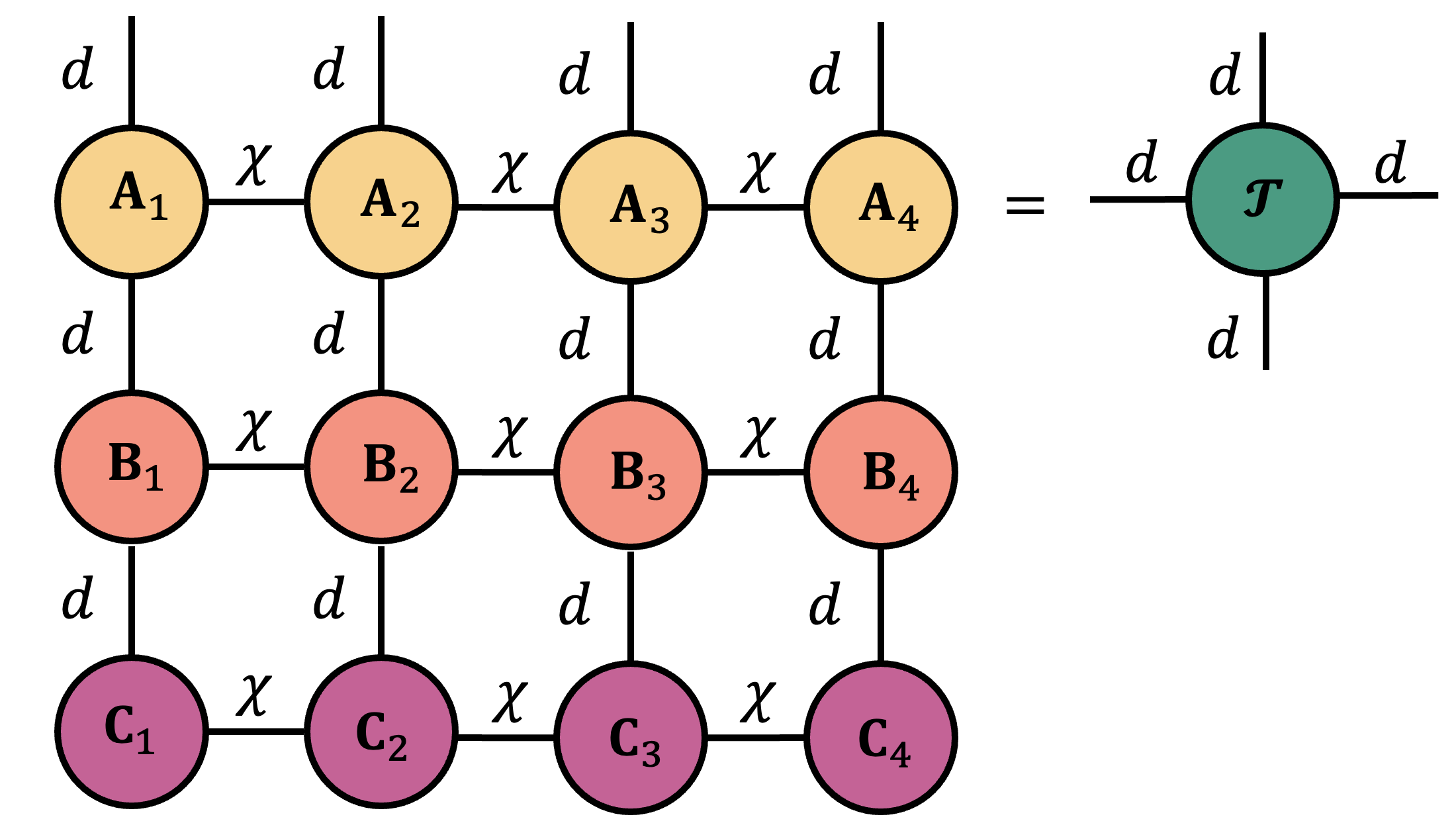
At this point, unless you have worked with Penrose diagrams before, the connection between the left and right columns in the example above is probably not yet obvious. Even so, this small example already shows how Penrose notation compresses information and keeps attention on the outcome of a large contraction rather than getting lost in Flander’s maze of indices.

What’s actually going on here? To understand tensor contraction, we need a way of adding modes and removing modes. Removing a shared mode during contraction should feel fairly intuitive: if two tensors share an index and we contract over it, that index should somehow be “deleted”.

To make this idea rigorous, we first need to understand how to place all modes from two tensors into a single ambient space.

Definition (Tensor Kronecker Product)

Let $\tX \in \Rtspace{n}$ be an order-$n$ tensor and let $\tY \in \bbR^{e_1 \times \cdots \times e_m}$ be an order-$m$ tensor. The Kronecker product of $\tX$ and $\tY$ is the order-$(n+m)$ tensor $$ \tX \otimes \tY \in \bbR^{d_1 \times \cdots \times d_n \times e_1 \times \cdots \times e_m}, \qquad (\tX \otimes \tY)(\vi,\vj) := \tX(\vi)\,\tY(\vj). $$

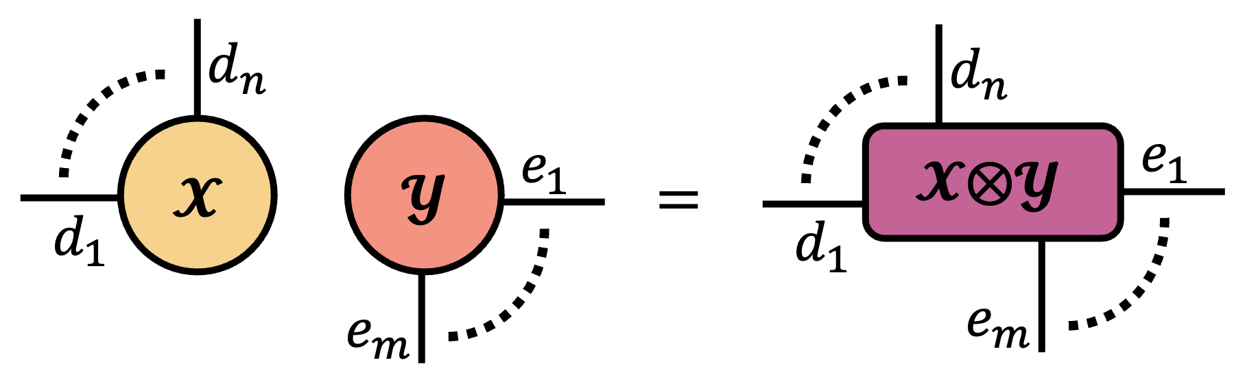
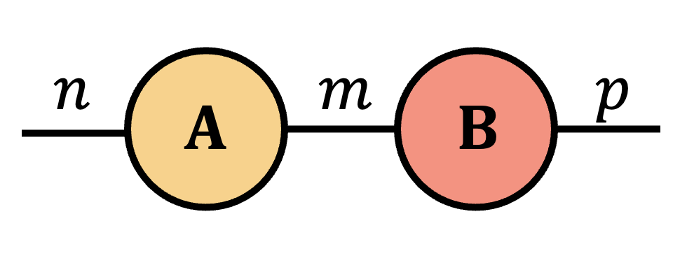
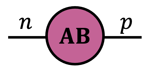
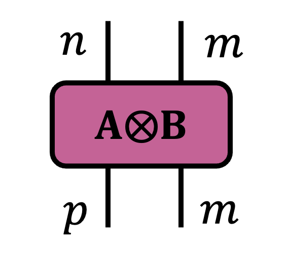
The notation $\tX(\vi)\,\tY(\vj)$ is shorthand here for $\tX(i_1\cdots i_n)\,\tY(j_1\cdots j_m)$. The tensor Kronecker product multiplies two tensors and retains all of their modes. In Penrose notation, the Kronecker product is represented by just placing two tensors next to one another.

When we instead want to remove modes, the operator of choice is the partial trace.

For matrices, the trace operator collapses an entire square matrix to a single scalar. Similarly, if two modes of a given tensor are the same, we can sum over their diagonal, leaving behind a scalar in their wake. Writing down this operation is a bit painful. As consolation, we will see in a moment that in Penrose diagrams this can be represented by drawing a single line.

Definition (Partial Trace of a Tensor)

Let $\tX \in \bbR^{d_1\times \cdots \times d_n}$, and choose indices $1\le \alpha<\beta\le n$ with $d_\alpha=d_\beta$. The partial trace over modes $\alpha$ and $\beta$ is obtained by setting those two indices equal and summing over their common value: $$ \operatorname{tr}_{\alpha,\,\beta}(\tX)(\vi_{<\alpha},\vi_{(\alpha,\beta)},\vi_{>\beta}) := \sum_{r=1}^{d_\alpha} \tX(\vi_{<\alpha},r,\vi_{(\alpha,\beta)},r,\vi_{>\beta}). $$ Here the output index tuple keeps every index except the $\alpha$th and $\beta$th: $$ (\vi_{<\alpha},\vi_{(\alpha,\beta)},\vi_{>\beta}) =(i_1,\dots,i_{\alpha-1},\,i_{\alpha+1},\dots,i_{\beta-1},\,i_{\beta+1},\dots,i_n). $$

TLDR: The partial trace replaces two mode indices that each range over $d_\alpha$ values with a single summation, producing a tensor with two fewer modes.

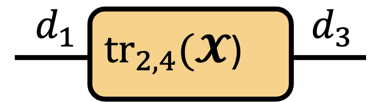
In Penrose notation, the partial trace is represented by drawing a connected line between two modes on the same tensor. Consider tracing over modes 2 and 4 of an order-4 tensor $\tX \in \bbR^{d_1\times d_2\times d_3\times d_4}$ with $d_2=d_4$.

\( \operatorname{tr}_{2,4} \) \(=\) \(=\)

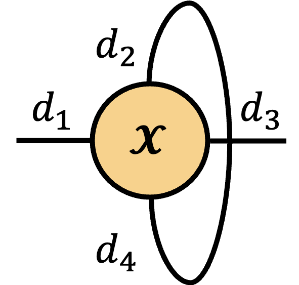Let’s also see what’s happening structurally when we take a partial trace.

My favorite part about this operator is that the classical notion of summing the diagonal of a matrix is preserved in the geometry of a given tensor.

Example: Partial Trace on a 3×4×3 Tensor

Let $\tX \in \bbR^{3\times 4\times 3}$. The partial trace over modes $1$ and $3$ sums the diagonal fibers $\tX(r, :, r)$ for $r=1,2,3$, producing a single vector in $\bbR^4$.

Instantiating the definition for $\tX \in \bbR^{3\times 4\times 3}$ (with $\alpha=1$, $\beta=3$) gives $$ \operatorname{tr}_{1,3}(\tX)(j) = \sum_{r=1}^{3}\tX(r,j,r), \qquad j\in[4]. $$ Here $\vi_{<\alpha}$ and $\vi_{>\beta}$ are empty, while $\vi_{(\alpha,\beta)}=(j)$. In the visualization, each diagonal fiber $\tX(r,:,r)$ is a $1\times 4$ vector, and their sum is a single vector. This is exactly what we should expect, since we removed two modes from an order-3 tensor.

Full 3×4×3 tensor

Isolated diagonal fibers $\tX(r,:,r)$

\( \operatorname{tr}_{1,3}(\tX)= \)

Fiber $r=1$

+

Fiber $r=2$

+

Fiber $r=3$

=

Partial trace result

With these two new operations in hand we are now prepared to define tensor contraction as the Kronecker product followed by a partial trace over the identified pair of modes.

Definition (Tensor Contraction)

Let $\tX \in \Rtspace{n}$ and $\tY \in \bbR^{e_1 \times \cdots \times e_m}$ share a mode size $d_\alpha=e_\beta$. The contraction of $\tX$ and $\tY$ along these modes, denoted $\tX \cp{\alpha}{\beta} \tY$, is the order-$(n+m-2)$ tensor obtained by taking a partial trace of their Kronecker product over the identified pair $$ \tX \cp{\alpha}{\beta} \tY := \operatorname{tr}_{\alpha,\,n+\beta}\bigl(\tX \otimes \tY\bigr). $$

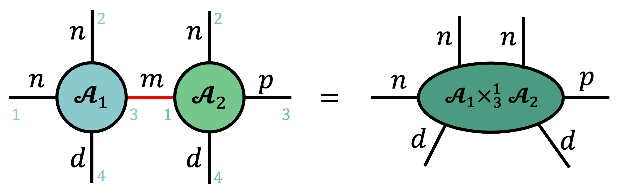
Example: Using the Contracted Product Operator

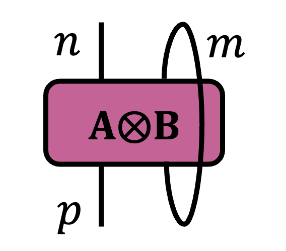
Below is an example of the contraction of a tensor $\tA_1\in \bbR^{n\times n\times m\times d}$ with another order-4 tensor $\tA_2\in \bbR^{m\times n\times p\times d}$ along their shared mode $m$, highlighted in red for convenience. Also shown is a choice of indexing convention for each tensor. In general, any ordering works as long as it is fixed throughout the analysis, though I typically use clockwise order starting at 9 o'clock (perhaps to the dismay of my friend Guifré Sánchez).

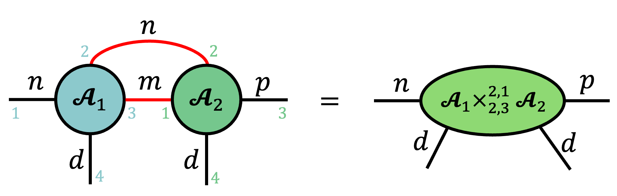
We can also define contractions over multiple modes simultaneously by writing tuples in the superscript and subscript of the contracted product operator.

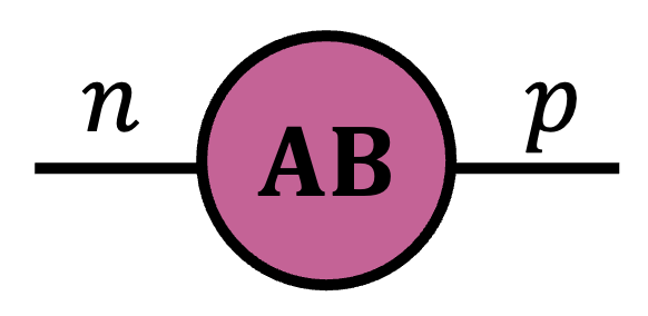
Defining tensor contraction this way is mathematically elegant, but it may not be immediately obvious how to recover simple contractions such as matrix multiplication. Below we show this example and detail how matrix multiplication can be derived as a simple sequence of Penrose diagrams following our definitions above.

Example: Matrix multiplication as tensor contraction

Proposition:

Let $\mA\in \bbR^{n\times m}$ and $\mB\in \bbR^{m\times p}$ be arbitrary real-valued matrices. The matrix product $\mA\mB$ can be written as $\mA\cp{2}{1}\mB$ and is represented by the following Penrose diagram.

=

Proof.

Traditional syntax

---

For $\mA\in \bbR^{n\times m}$ and $\mB\in \bbR^{m\times p}$, write $$ \begin{aligned} \mA&=\sum_{i,j}\mA(i,j)\,(\ve_i\otimes \ve_j),\\ \mB&=\sum_{k,\ell}\mB(k,\ell)\,(\ve_k\otimes \ve_\ell). \end{aligned} $$ By the contraction definition, $$ \begin{aligned} \mA\cp{2}{1}\mB &= \operatorname{tr}_{2,1}(\mA\otimes\mB) \\ &= \operatorname{tr}_{2,1}\!\left[\sum_{i,j,k,\ell}\mA(i,j)\,\mB(k,\ell)\, \ve_i\otimes \ve_j\otimes \ve_k\otimes \ve_\ell\right] \\ &= \sum_{i,j,k,\ell}\mA(i,j)\,\mB(k,\ell)\, \operatorname{tr}_{2,1}\!\left(\ve_i\otimes \ve_j\otimes \ve_k\otimes \ve_\ell\right). \end{aligned} $$ Using $$ \begin{aligned} \operatorname{tr}_{2,1}\!\left(\ve_i\otimes \ve_j\otimes \ve_k\otimes \ve_\ell\right) &=\langle \ve_j,\ve_k\rangle\,\ve_i\otimes \ve_\ell \\ &=\delta_{jk}\,\ve_i\otimes \ve_\ell, \end{aligned} $$ we get $$ \begin{aligned} \mA\cp{2}{1}\mB &= \sum_{i,j,\ell}\mA(i,j)\,\mB(j,\ell)\,\ve_i\otimes \ve_\ell \\ &= \sum_{i,\ell}\left(\sum_j\mA(i,j)\,\mB(j,\ell)\right)\ve_i\otimes \ve_\ell \\ &= \sum_{i,\ell}(\mA\mB)(i,\ell)\,\ve_i\otimes \ve_\ell = \mA\mB. \end{aligned} $$

Penrose notation

---

$\mA$ and $\mB$ next to each other

Tensor Kronecker product

Partial trace

Solution

The Payoff: Computational Complexity At A Glance

Now that we have defined Penrose diagrams and formalized what they communicate, I want to highlight one of my favorite consequences of this notation: it provides a direct way to reason about computational complexity when designing linear algebra algorithms.

I first learned this fact from Ethan Epperly some time around July 2023, and it has reshaped how I approach linear algebra and algorithm design. The main idea is the following.

The cost of a single tensor contraction is proportional to the product of the dimensions of all indices that appear in that contraction.

This fact is known in certain corners of the theoretical computer science community concerned with multilinear algebra [pg. 4, 8], and is somewhat immediate once we recognize that contracting two tensors requires accessing all involved entries. Over the last few years, I have started to see it appear more frequently in papers on tensor network methods [10, Figs. 7-9] an I antcipate this idea becoming increasingly standard for analyzing the runtime of tensor network algorithms.

Let’s apply this idea to some contractions we have already seen in this blog post. For each contraction we just write down a big O statement containing the product of all the modes involved.

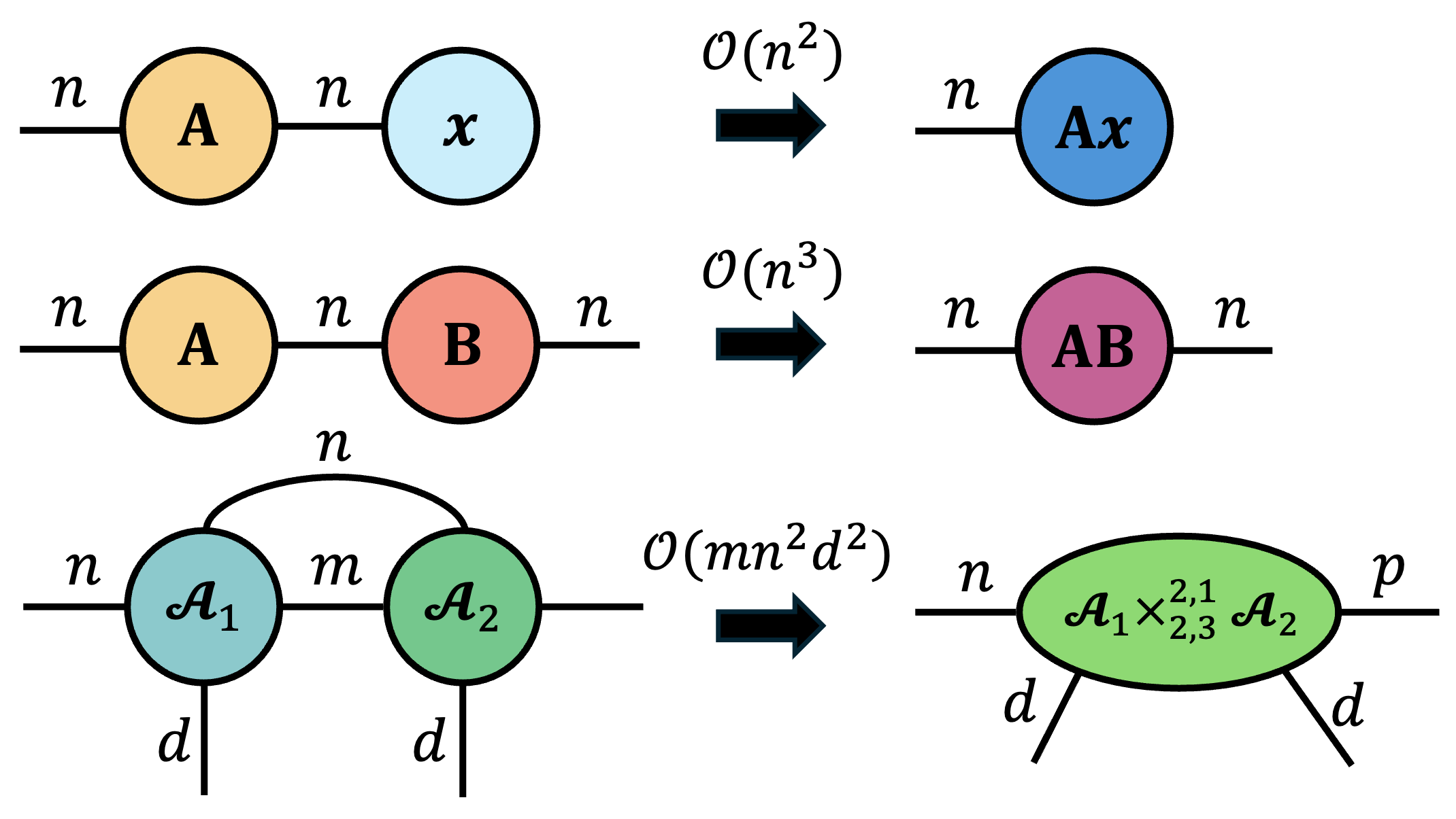
As we can see, we can recover naive bounds for matrix multiplication and matrix-vector multiplication, and we can also quickly recover the cost of a fairly specific tensor contraction.

Things become particularly interesting when we place assumptions on the typical size of the modes of a given tensor. Consider the cost of contracting together the following Penrose diagram.

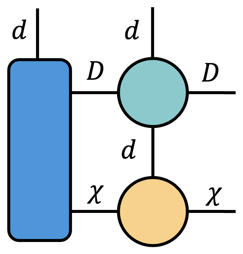
Depending on the order in which we contract the tensors, we generate different intermediate tensor sizes, which changes the total asymptotic time complexity of the contraction. For instance, here are two contraction sequences that arrive at the same result but have different time complexity.

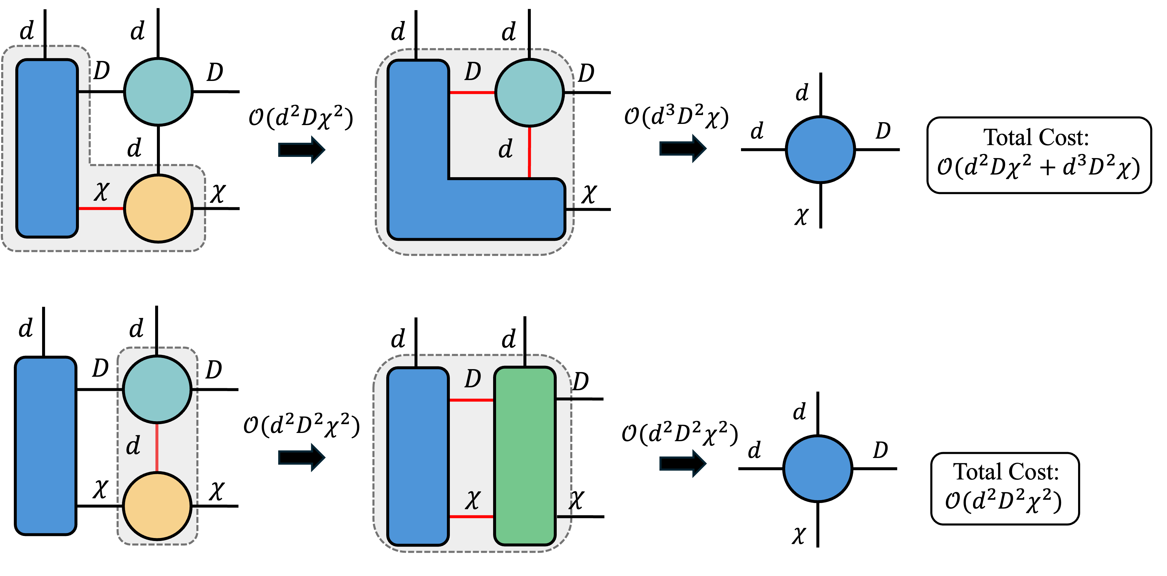
Depending on the relationship between the mode dimensions $d$, $D$, and $\chi$, one of these contraction sequences may be cheaper than another. This specific contraction example above appears very frequently in various tensor network algorithms such as MPO-MPS products, DMRG and others.

In general, identifying optimal tensor contraction sequences is NP-hard [11].Identifying general-purpose approximate tensor contraction sequences is an active research area (see, for example, [12]). Luckily, in many small-scale examples like the one above, the search space is still tractable (and often fairly straightforward to think about), so near-optimal or optimal contraction paths can often be found a priori to develop fast algorithms.

I work in the field of randomized linear algebra, and my research is primarily focused on how randomization can be used for accelerating and developing new tensor network methods.

Both of these fields gain leverage over exact methods by compressing information. Perhaps unsurprisingly, I enjoy Penrose notation for exactly the same reason. The ability to compress tensor operations down to circles and lines is dramatically liberating, and has allowed me to make progress on research problems at a greatly accelerated pace.

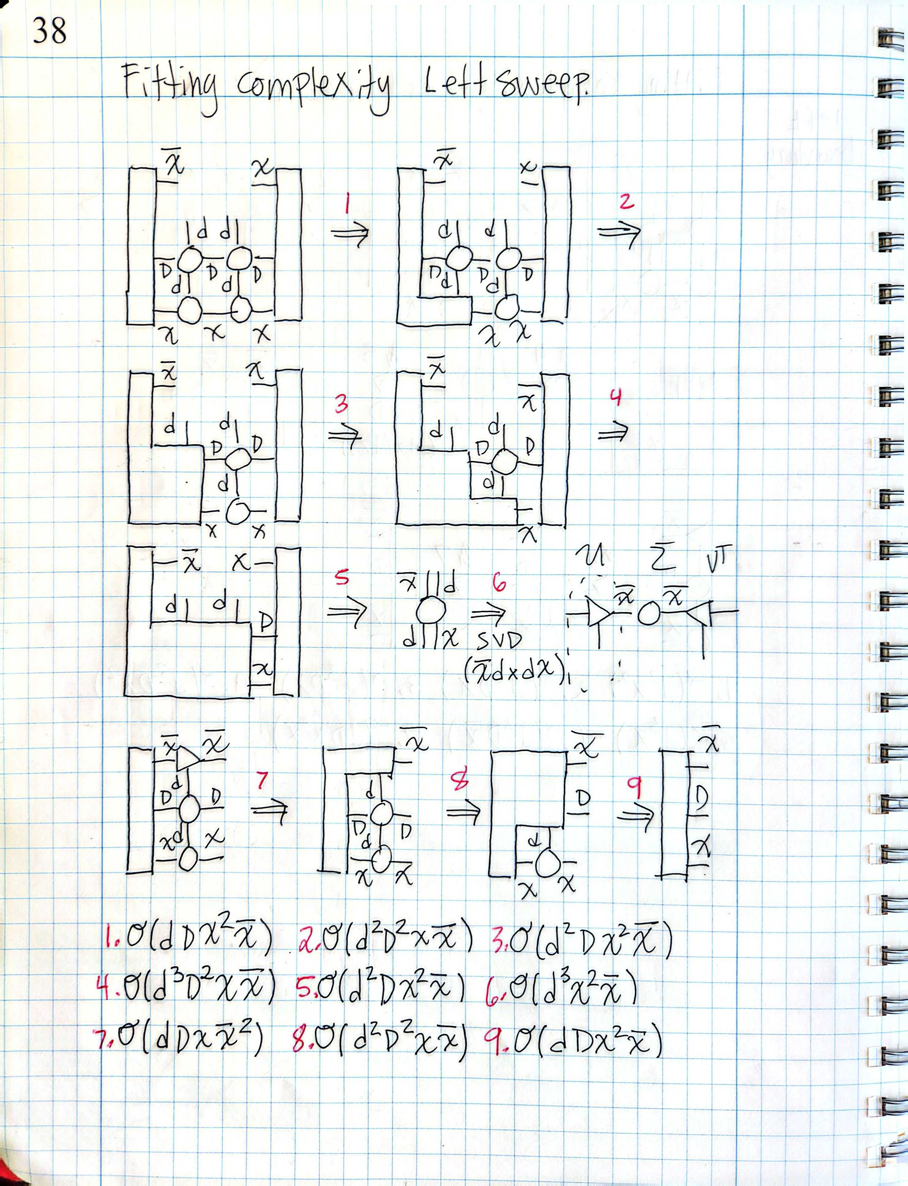
For example, the image on the left is an excerpt from one of my notebooks containing an asymptotic complexity analysis of the tensor contractions within the two-site Fitting (variational) algorithm for the compressed MPO-MPS product [13], which I conducted while working on Successive Randomized Compression (SRC) [14].

This page may have taken about 10 minutes to draw, and it quickly delivered an estimate of how expensive this algorithm was. If I had instead attempted to write a formal analysis in traditional syntax, I am not sure that I would have been brave enough to finish.

In summary, Penrose diagrams are an alternative syntax for thinking about tensor contraction, annd make it very easy to think about tensor algorithms and operations. Hopefully the content of this blog post encourages you to try out Penrose diagrams in your own work, particularly if you are a research scientist studying these methods.

References

- , “The ubiquitous Kronecker product” , Journal of Computational and Applied Mathematics , vol. 123 , no. 1 , pp. 85-100 , 2000 , doi: https://doi.org/10.1016/S0377-0427(00)00393-9 .
- , “Matrix computations” , JHU press , 2013 .
- , “Differential forms with applications to the physical sciences” , Courier Corporation , vol. 11 , 1963 .
- , “Randomized algorithms for streaming low-rank approximation in tree tensor network format” , arXiv preprint arXiv:2412.06111 , 2024 .
- , “Applications of negative dimensional tensors” , Combinatorial mathematics and its applications , vol. 1 , no. 221-244 , pp. 3 , 1971 .
- , “The Tensor Cookbook” , 2024 , https://tensorcookbook.com .
- , “Tensor Decompositions for Data Science” , Cambridge University Press , 2025 .
- , “Hand-waving and interpretive dance: an introductory course on tensor networks” , Journal of Physics A: Mathematical and Theoretical , vol. 50 , no. 22 , pp. 223001 , 2017 , doi: 10.1088/1751-8121/aa6dc3 .
- , “An introduction to graphical tensor notation for mechanistic interpretability” , arXiv preprint arXiv:2402.01790 , 2024 .
- , “Approximate Contraction of Arbitrary Tensor Networks with a Flexible and Efficient Density Matrix Algorithm” , Quantum , vol. 8 , pp. 1580 , 2024 , doi: 10.22331/q-2024-12-27-1580 .
- , “NP-Hardness of Tensor Network Contraction Ordering” , 2023 , https://arxiv.org/abs/2310.06140 .
- , “Hyper-optimized tensor network contraction” , Quantum , vol. 5 , pp. 410 , 2021 , doi: 10.22331/q-2021-03-15-410 .
- , “Renormalization algorithms for Quantum-Many Body Systems in two and higher dimensions” , 2004 , https://arxiv.org/abs/cond-mat/0407066 .
- , “Successive randomized compression: A randomized algorithm for the compressed MPO-MPS product” , 2026 , https://arxiv.org/abs/2504.06475 .
Last updated: February 22, 2026
Comments
Leave a new comment